Example file of how to use adaptive sparse grid for HJB Equation

by SeHyoun Ahn, July 2016

Set up Grids
Set up Model
Iterate to Solve HJB Equation Adding Nodes to Sparse Grids as Needed
Comparison Plot to Full Grid

% Requires: <generate_spgrid.m>
%
%           <gen_diff_op.m>
%
%           <grid_evaluation.m>
%

Set up Grids

n_dim = 2;                 % Dimensionality of the problem
n_levels = 4;              % Level of the starting sparse grid
I = 100;                   % Number of asset grid points for full grid
J = 40;                    % Number of skill grid points for full grid

% Generate sparse grid
[spgrid,spspace] = generate_spgrid(n_dim,n_levels);


% Setup Change of basis from Hierachical to Nodal
hier_to_nodal = grid_evaluation(spgrid,spgrid,spspace);

% Generate Difference Operators
[forward_diff_x,backward_diff_x] = gen_diff_op(1,spgrid,spspace,min(spspace(:,1)));
[forward_diff_y,backward_diff_y] = gen_diff_op(2,spgrid,spspace,min(spspace(:,2)));

% Second Derivative Operator
% More tests are needed to check which stencil is the best for second order
% Operators
second_deriv_y = forward_diff_y*(hier_to_nodal\backward_diff_y) ...
  + backward_diff_y*(hier_to_nodal\forward_diff_y);
second_deriv_y(spgrid(:,2)==1,:) = -backward_diff_y(spgrid(:,2)==1,:);
second_deriv_y(spgrid(:,2)==0,:) = forward_diff_y(spgrid(:,2)==0,:);

% Integration Weights
% This does not get used here
int_weight = (prod(spspace,2)./2.^sum(spspace==1,2))';

Set up Model

Parameters

ga = 2;             % CRRA utility with parameter gamma
alpha = 0.35;       % Production function F = K^alpha * L^(1-alpha)
delta = 0.1;        % Capital depreciation
zmean = 1.0;        % mean O-U process (in levels). This parameter has to be adjusted to ensure that the mean of z (truncated gaussian) is 1.
sig2 = (0.10)^2;    % sigma^2 O-U
Corr = exp(-0.3);   % persistence -log(Corr)  O-U
rho = 0.05;         % discount rate
TFP = 1;

K = 3.8;            % initial aggregate capital. It is important to guess a value close to the solution for the algorithm to converge

zmin = 0.5;   % Range z
zmax = 1.5;
amin = -1;    % borrowing constraint
amax = 30;    % range a

%simulation parameters
maxit  = 100;       %maximum number of iterations in the HJB loop
maxitK = 100;       %maximum number of iterations in the K loop
crit = 10^(-10);    %criterion HJB loop
critK = 1e-7;       %criterion K loop
Delta = 1000;       %delta in HJB algorithm

% Ornstein-Uhlenbeck
the = -log(Corr);
Var = sig2/(2*the);

% Evalute asset and skill values for grid points
aa = spgrid(:,1)*(amax-amin)+amin;
zz = spgrid(:,2)*(zmax-zmin)+zmin;
mu = the*(zmean-zz);
s2 = sig2;

% Differential operator for skill
Aswitch = bsxfun(@times,mu.*(mu>=0),forward_diff_y)/(zmax-zmin) ...
  + bsxfun(@times,mu.*(mu<0),backward_diff_y)/(zmax-zmin) ...
  + s2/2*second_deriv_y/(zmax-zmin)^2;

% Initial guess
r = alpha     * TFP * K^(alpha-1) -delta; %interest rates
w = (1-alpha) * TFP * K^(alpha);          %wages
v0 = (w.*zz + r.*aa).^(1-ga)/(1-ga)/rho;
v = hier_to_nodal\v0;
dist = zeros(1,maxit);
V=v;

number_of_points=0;

Iterate to Solve HJB Equation Adding Nodes to Sparse Grids as Needed

Note that the Iteration Part of the Code is the same except for difference operator

while true

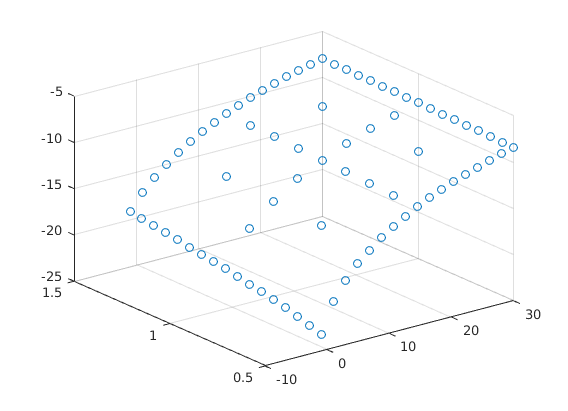
  for n=1:maxit
    Vaf = forward_diff_x*V/(amax-amin);
    Vab = backward_diff_x*V/(amax-amin);

    c0 = w*zz + r.*aa;
    cf = Vaf.^(-1/ga);
    sf = w*zz + r.*aa - cf;
    cb = Vab.^(-1/ga);
    sb = w*zz + r.*aa - cb;

    If = (sf >  0).*(spgrid(:,1)<1);
    Ib = (sb < 0).*(If==0).*(spgrid(:,1)>0);
    I0 = (1-If-Ib);

    c = cf.*If + cb.*Ib + c0.*I0;
    u = c.^(1-ga)/(1-ga);

    AA = bsxfun(@times,If.*sf,forward_diff_x)/(amax-amin) + bsxfun(@times,Ib.*sb,backward_diff_x)/(amax-amin);

    B = (1/Delta + rho)*hier_to_nodal - AA - Aswitch;

    b = u + hier_to_nodal*V/Delta;

    V_new = B\b;

    Vchange = V_new - V;
    V = V_new;

    dist = max(max(abs(Vchange)));
    if dist<crit
      disp('Value Function Converged, Iteration = ')
      disp(n)
      break
    end
  end

  % Plot Value function given the grid
  figure(1);
  scatter3(aa,zz,hier_to_nodal*V);
  drawnow;

  V_nodal = hier_to_nodal*V;

Value Function Converged, Iteration = 
     9

Add new nodes to sparse grid if needed

  % Find Position to Expand
  loc = abs(V)>1e-4*(max(V_nodal)-min(V_nodal));

  % Compute New Grid Points from active grid points
  [new_points,new_spaces] = gen_new_points(spgrid(loc,:),spspace(loc,:));

  % Find Positions to Compress Away
  loc_keep = abs(V)>8e-5*(max(V_nodal)-min(V_nodal));
  [xx,loc] = unique([spgrid(loc_keep,:);new_points],'rows');

  % Break if no new grid points are added
  if number_of_points >= size(xx,1)
    break;
  end
  number_of_points = size(xx,1);

  % Update interpolation operator
  x_eval = grid_evaluation(xx,spgrid,spspace);
  v_nodal = x_eval*V;
  spgrid = xx;
  spspace = [spspace(loc_keep,:);new_spaces];
  spspace = spspace(loc,:);
  hier_to_nodal = grid_evaluation(xx,spgrid,spspace);

  % Correct the basis function for the new bases
  V = hier_to_nodal\v_nodal;

  % Update Difference Operators for the new grid
  [forward_diff_x,backward_diff_x] = gen_diff_op(1,spgrid,spspace,min(spspace(:,1)));
  [forward_diff_y,backward_diff_y] = gen_diff_op(2,spgrid,spspace,min(spspace(:,2)));
  second_deriv_y = forward_diff_y*(hier_to_nodal\backward_diff_y) ...
    + backward_diff_y*(hier_to_nodal\forward_diff_y);
  second_deriv_y(spgrid(:,2)==1,:) = -backward_diff_y(spgrid(:,2)==1,:);
  second_deriv_y(spgrid(:,2)==0,:) = forward_diff_y(spgrid(:,2)==0,:);

  % Update Nodal Values for new grid
  aa = spgrid(:,1)*(amax-amin)+amin;
  zz = spgrid(:,2)*(zmax-zmin)+zmin;
  mu = the*(zmean-zz);
  s2 = sig2;

  Aswitch = bsxfun(@times,mu.*(mu>=0),forward_diff_y)/(zmax-zmin) ...
    + bsxfun(@times,mu.*(mu<0),backward_diff_y)/(zmax-zmin) ...
    + s2/2*second_deriv_y/(zmax-zmin)^2;

end

  Value Function Converged, Iteration = 
     7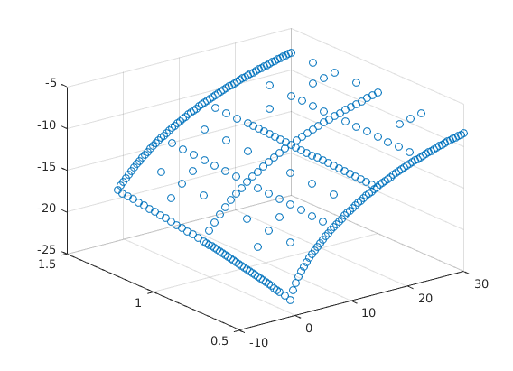

 Value Function Converged, Iteration = 
     8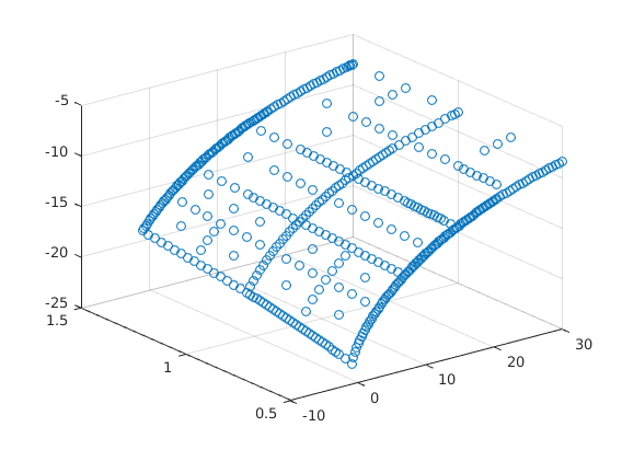

 Value Function Converged, Iteration = 
     8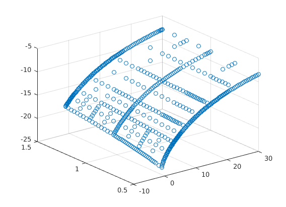

 Value Function Converged, Iteration = 
     9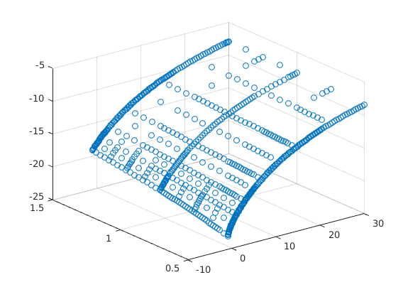

 Value Function Converged, Iteration = 
     8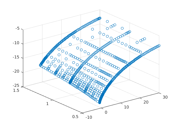

 Value Function Converged, Iteration = 
     8

 Value Function Converged, Iteration = 
     7

 Value Function Converged, Iteration = 
     6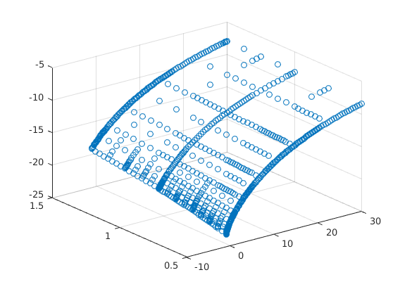

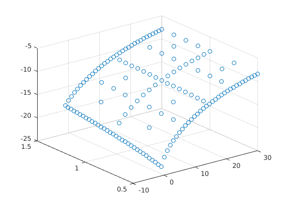
 Value Function Converged, Iteration = 
     7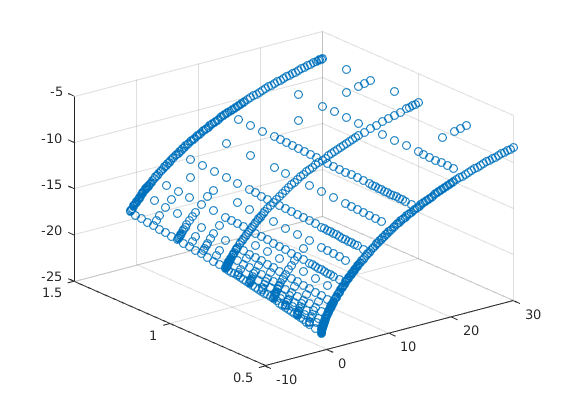

 
figure(2);
scatter3(aa,zz,hier_to_nodal*V);
V_sparse = V;

 Comparison Plot to Full Grid
The following code is adapted from Ben Moll's codes available at     https://www.princeton.edu/~moll/HACTproject.htm
a = linspace(amin,amax,I)';    % wealth vector
da = (amax-amin)/(I-1);
z = linspace(zmin,zmax,J);     % productivity vector
dz = (zmax-zmin)/(J-1);
dz2 = dz^2;
aa = a*ones(1,J);
zz = ones(I,1)*z;

mu = the*(zmean - z);        % Drift
s2 = sig2.*ones(1,J);        % Variance

% Preallocation
Vaf = zeros(I,J);
Vab = zeros(I,J);
Vzf = zeros(I,J);
Vzb = zeros(I,J);
Vzz = zeros(I,J);
c = zeros(I,J);

yy = - s2/dz2 - mu/dz;
chi =  s2/(2*dz2);
zeta = mu/dz + s2/(2*dz2);

updiag=zeros(I*J,1); %This is necessary because of the peculiar way spdiags is defined.
updiag(I+1:I*J)=reshape(repmat(zeta(1:J-1),I,1),I*(J-1),1);

centdiag=zeros(I*J,1);
centdiag(1:I)=repmat(chi(1)+yy(1),I,1);
centdiag(I+1:I*(J-1))=reshape(repmat(yy(2:J-1),I,1),I*(J-2),1);
centdiag(I*J-I+1:I*J)=repmat(yy(J)+zeta(J),I,1);

lowdiag=reshape(repmat(chi(2:J),I,1),I*(J-1),1);

Aswitch=spdiags(centdiag,0,I*J,I*J)+spdiags(lowdiag,-I,I*J,I*J)+spdiags(updiag,I,I*J,I*J);

% Initial Guess
r = alpha     * TFP * K^(alpha-1) -delta; %interest rates
w = (1-alpha) * TFP * K^(alpha);          %wages
v0 = (w*zz + r.*aa).^(1-ga)/(1-ga)/rho;
v = v0;

for n=1:maxit
  V = v;

  % forward difference
  Vaf(1:I-1,:) = (V(2:I,:)-V(1:I-1,:))/da;
  Vaf(I,:) = (w*z + r.*amax).^(-ga); %will never be used, but impose state constraint a<=amax just in case

  % backward difference
  Vab(2:I,:) = (V(2:I,:)-V(1:I-1,:))/da;
  Vab(1,:) = (w*z + r.*amin).^(-ga);  %state constraint boundary condition

  %consumption and savings with forward difference
  cf = Vaf.^(-1/ga);
  sf = w*zz + r.*aa - cf;
  %consumption and savings with backward difference
  cb = Vab.^(-1/ga);
  sb = w*zz + r.*aa - cb;
  %consumption and derivative of value function at steady state
  c0 = w*zz + r.*aa;
  Va0 = c0.^(-ga);

  If = sf > 0; %positive drift --> forward difference
  Ib = sb < 0; %negative drift --> backward difference
  I0 = (1-If-Ib); %at steady state

  Va_Upwind = Vaf.*If + Vab.*Ib + Va0.*I0; %important to include third term

  c = Va_Upwind.^(-1/ga);
  u = c.^(1-ga)/(1-ga);

  X = - min(sb,0)/da;
  Y = - max(sf,0)/da + min(sb,0)/da;
  Z = max(sf,0)/da;

  Z(I,:)=0;
  X(1,:)=0;
  updiag=[0;reshape(Z,I*J,1)];
  centdiag=reshape(Y,I*J,1);
  lowdiag=reshape(X,I*J,1);

  AA=spdiags(centdiag,0,I*J,I*J)+spdiags([updiag;0],1,I*J,I*J)+spdiags(lowdiag(2:I*J),-1,I*J,I*J);
  A = AA + Aswitch;
  B = (1/Delta + rho)*speye(I*J) - A;

  u_stacked = reshape(u,I*J,1);
  V_stacked = reshape(V,I*J,1);

  b = u_stacked + V_stacked/Delta;

  V_stacked = B\b;

  V = reshape(V_stacked,I,J);

  Vchange = V - v;
  v = V;

  dist = max(max(abs(Vchange)));
  if dist<crit
    disp('Value Function Converged with Full Grid, Iteration = ');
    disp(n);
    break;
  end
end

h = figure(2);
hold on;
surf(a,z,V');
title('Comparison to Uniform Grid');
gif_maker_rotate('comparison.gif',h);
Value Function Converged with Full Grid, Iteration = 
     8

 
Published with MATLAB® R2016a
 (and adjusted not to clash with Bootstrap)

Example file of how to use adaptive sparse grid for HJB Equation

Contents

Set up Grids

Set up Model

Iterate to Solve HJB Equation Adding Nodes to Sparse Grids as Needed

Comparison Plot to Full Grid