Solves the Krusell and Smith (1998)

Solving Krusell-Smith model using perturbation method involves simple 5 step process given by

In this example file, the entire problem will be solved total of 3 times. First, KS model will be solved without any model reduction. Second, KS model will be solved with model reduction, to compare how well the model reduction works. Lastly, different parts of observables will be introduced to compare how the model reduction works with different requirements. We have updates to Internal Consistency check coming in the future.

Estimated Runtime: 1.5 seconds

REFERENCES:

REQUIRES:

Relevant files except for auto diff toolbox, can be found in /examples/KrusellSmith folder of phact toolbox provided on github

Contents

Setup the toolbox

Just need to include folders containing the files in the path.

addpath('/path/to/autodiff/toolbox/');
addpath('/path/to/phact/toolbox');

Set options for this example run

example_case : 1 run full and compare with only value function reduction 2 run full and compare with only state space reduction 3 run full and compare with both reductions

example_case = 3;
reduceDist_hor = 50;        % m of K_m(A,b)

% initialize shocks for simulation
T = 200;
N = 2000;
vAggregateShock = zeros(1,N);
vAggregateShock(1,1) = 1;
%vAggregateShock = randn(1,N);     % Uncomment for one realization instead
                                  % of IRFs

Step 0: Set Parameters

The script sets up parameters relevant for the model

set_parameters;

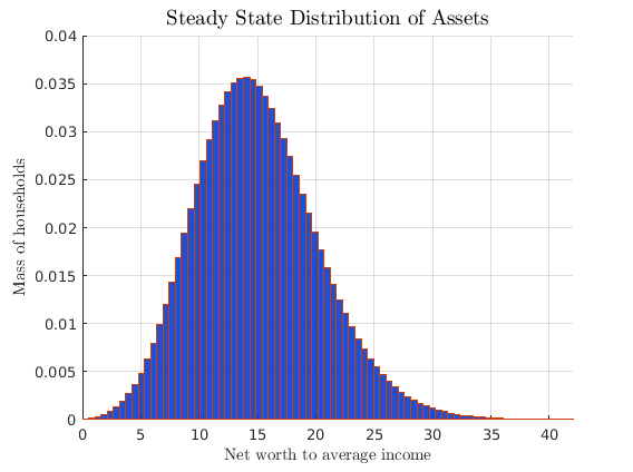
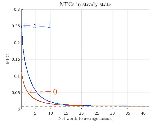
Step 1: Solve for Steady State

Non-stochastic steady state can be found using any methods. In particular, example codes can be found at http://www.princeton.edu/~moll/HACTproject.htm.

tStart = tic;
fprintf('Computing steady state...\n')
global IfSS IbSS I0SS varsSS A

[rSS,wSS,KSS,ASS,uSS,cSS,VSS,gSS,dVUSS,dVfSS,dVbSS,IfSS,IbSS,I0SS] = ...
    compute_steady_state();

fprintf('Time to compute steady state: %.3g seconds\n\n\n',toc(tStart));

% Store steady state values
varsSS = zeros(nVars,1);
varsSS(1:2*I,1) = reshape(VSS,2*I,1);
ggSS = reshape(gSS,2*I,1);
varsSS(2*I+1:4*I-1,1) = ggSS(1:2*I-1);
varsSS(4*I,1) = 0;
varsSS(4*I+1,1) = KSS;
varsSS(4*I+2,1) = rSS;
varsSS(4*I+3,1) = wSS;
varsSS(4*I+4,1) = (KSS ^ aalpha) * (zAvg ^ (1 - aalpha));
CSS = sum(cSS(:) .* gSS(:) * da);
varsSS(4*I+5,1) = CSS;
varsSS(4*I+6,1) = ddelta * KSS;

% plot steady state results
plot_steady_state;

Computing steady state...
Steady State Found, Interest rate =
    0.0096

Time to compute steady state: 0.128 seconds

Step 2: Linearize Model Equations

For computing derivatives, the codes written for solving for the steady-state can be used almost verbatim using automatic differentiation toolbox as long as only the functions supported by automatic differentation are used. For list of supported functions and documentation of relevant syntax check https://github.com/sehyoun/MATLABAutoDiff. Example usage/syntax of automatic differentiation can be found at http://sehyoun.com/EXAMPLE_AutoDiff_Syntax.html

fprintf('Taking derivatives of equilibrium conditions...\n')
t0 = tic;

% Prepare automatic differentiation
vars = zeros(2*nVars+nEErrors+1,1);
vars = myAD(vars);

% Evaluate derivatives
derivativesIntermediate = equilibrium_conditions(vars);

% Extract out derivative values
derivs = getderivs(derivativesIntermediate);

tDerivs = toc(t0);
fprintf('...Done!\n')
fprintf('Time to compute derivatives: %2.4f seconds\n\n\n',tDerivs)
if tDerivs > 1
    warning('If you do not compile mex files for automatics differentiation, matrix vector multiplication will be slow');
    disp('Press any key to continue...');
    pause();
end

% Unpackage derivatives
mVarsDerivs = derivs(:,1:nVars);
mVarsDotDerivs = derivs(:,nVars+1:2*nVars);
mEErrorsDerivs = derivs(:,2*nVars+1:2*nVars+nEErrors);
mShocksDerivs = derivs(:,2*nVars+nEErrors+1);

Taking derivatives of equilibrium conditions...
...Done!
Time to compute derivatives: 0.0390 seconds

Step 3 (full): Solve out Static Constraints and/or Reduce Models

For the first run, a unreduced model will be solved

% rename derivative matrix to match notation in paper
g0 = mVarsDotDerivs;
g1 = -mVarsDerivs;
c = sparse(nVars,1);
psi = -mShocksDerivs;
pi = -mEErrorsDerivs;

% Solve out static constratins
[~,inv_state_red,g0,g1,constant,pi,psi] = clean_G0_sparse(g0,g1,c,pi,psi);

Step 4: Solve Linear System

t0 = tic;
fprintf('Solving linear system...\n')

[G1,~,impact,eu] = schur_solver(g0,g1,c,psi,pi,1,1,1);

fprintf('...Done!\n')
fprintf('Existence and uniqueness? %2.0f and %2.0f\n',eu);
fprintf('Time to solve full linear system: %2.4f seconds\n\n\n',toc(t0))

Solving linear system...
...Done!
Existence and uniqueness?  1 and  1
Time to solve full linear system: 0.1721 seconds

Step 5: Simulate Impulse Response Functions

t0 = tic;

[simulated,~] = simulate(G1,impact,T,N,vAggregateShock,'implicit',inv_state_red);%,4*I:4*I+6);

fprintf('...Done!\n')
fprintf('Time to simulate model: %2.4f seconds\n\n\n',toc(t0))

big_simul = simulated + varsSS;
simulated = simulated(4*I:4*I+6,:);

varsSS_small = varsSS(4*I:4*I+6,1);
% Add state-states back in to get values in levels
vAggregateTFP			= simulated(1,:) + varsSS_small(1);
vAggregateOutput		= simulated(5,:) + varsSS_small(5);
vAggregateConsumption	= simulated(6,:) + varsSS_small(6);
vAggregateInvestment 	= simulated(7,:) + varsSS_small(7);

% Compute log differences for plotting
vAggregateTFP_full		= vAggregateTFP;
vAggregateOutput_full	= log(vAggregateOutput) - log(varsSS_small(5));
vAggregateConsumption_full	= log(vAggregateConsumption) - log(varsSS_small(6));
vAggregateInvestment_full	= log(vAggregateInvestment) - log(varsSS_small(7));

...Done!
Time to simulate model: 0.1098 seconds

Step 3 (reduced): Solve Out Static Constraints and/or Reduce Models

% Set relevant parameters for example cases
if (example_case == 1)
    reduceV = 1;
    reduceDistribution = 0;
elseif (example_case == 2)
    reduceV = 0;
    reduceDistribution = 1;
else
    reduceV = 1;
    reduceDistribution = 1;
end

% rename derivatives to match notation in paper
g0 = mVarsDotDerivs;
g1 = -mVarsDerivs;
c = sparse(nVars,1);
psi = -mShocksDerivs;
pi = -mEErrorsDerivs;

t0 = tic;
fprintf('Model Reduction ...\n')

Model Reduction ...

State space reduction using Krylov subspace method

if reduceDistribution == 1
    % State space reduction
    [state_red,inv_state_red,n_g_red] = krylov_reduction(g0,g1,n_v,n_g,reduceDist_hor);
    [g1,psi,pi,c,g0] = change_basis(state_red,inv_state_red,g1,psi,pi,c,g0);
else
    % Clean G0
    [state_red,inv_state_red,g0,g1,c,pi,psi] = clean_G0_sparse(g0,g1,c,pi,psi);
    n_g_red = n_g;
end

Value function reduction using spline inspired bases

if reduceV == 1
    % Create knot points for spline (the knot points are not uniformly spaced)
    knots = linspace(amin,amax,n_knots-1)';
    knots = (amax-amin)/(2^c_power-1)*((knots-amin)/(amax-amin)+1).^c_power+amin-(amax-amin)/(2^c_power-1);
    % Function calls to create basis reduction
    [from_spline, to_spline] = oneDquad_spline(x,knots);
    [from_spline, to_spline] = extend_to_nd(from_spline,to_spline,n_prior,n_post);
    n_splined = size(from_spline,2);
    [from_spline, to_spline] = projection_for_subset(from_spline,to_spline,0,n_g_red);

    % Reduce the decision vector
    [g1,psi,~,c,g0] = change_basis(to_spline,from_spline,g1,psi,pi,c,g0);
    pi = to_spline * pi * from_spline(1:n_v,1:n_splined);
elseif reduceV == 0
    from_spline = speye(n_g_red + n_v);
    to_spline = speye(n_g_red + n_v);
    n_splined = n_v;
end
fprintf('...Done!\n')
fprintf('Time to reduce dimensionality: %2.4f seconds\n\n\n',toc(t0))

...Done!
Time to reduce dimensionality: 0.1048 seconds

Step 4: Solve Linear System

t0 = tic;
fprintf('Solving reduced linear system...\n')

[G1,~,impact,eu,F] = schur_solver(g0,g1,c,psi,pi,1,1,1);

fprintf('...Done!\n')
fprintf('Existence and uniqueness? %2.0f and %2.0f\n',eu);
fprintf('Time to solve linear system: %2.4f seconds\n\n\n',toc(t0))

Solving reduced linear system...
...Done!
Existence and uniqueness?  1 and  1
Time to solve linear system: 0.0057 seconds

Step 5: Simulate Impulse Response Functions

fprintf('Simulating Model...\n')
t0 = tic;

trans_mat = inv_state_red*from_spline;
[simulated,vTime] = simulate(G1,impact,T,N,vAggregateShock,'implicit',trans_mat,4*I:4*I+6);

fprintf('...Done!\n')
fprintf('Time to simulate model: %2.4f seconds\n\n\n',toc(t0))

% Add state-states back in to get values in levels
vAggregateTFP = simulated(1,:) + varsSS_small(1);
vAggregateOuput = simulated(5,:) + varsSS_small(5);
vAggregateConsumption = simulated(6,:) + varsSS_small(6);
vAggregateInvestment = simulated(7,:) + varsSS_small(7);

% Compute log differences for plotting
vAggregateTFP_reduced = vAggregateTFP;
vAggregateOutput_reduced = log(vAggregateOutput) - log(varsSS_small(5));
vAggregateConsumption_reduced = log(vAggregateConsumption) - log(varsSS_small(6));
vAggregateInvestment_reduced = log(vAggregateInvestment) - log(varsSS_small(7));

Simulating Model...
...Done!
Time to simulate model: 0.0467 seconds

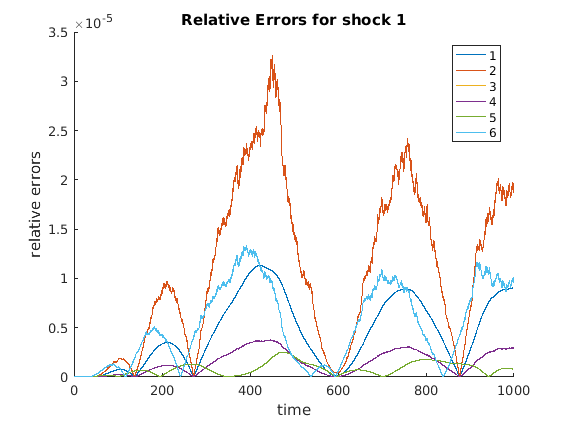
Step 6: Internal Consistency Check

For large problem, we are forced to take explicit update, so it can take awhile to run, but the good thing is that this only needs to be run at the end. We are currently working on this, so speed for this part might improve in the future. (For small problems, the speed is not an issue). A different consistency check is in works, and will be updated in the future.

g1 = -mVarsDerivs;
psi = -mShocksDerivs;
from_red = inv_state_red * from_spline;
to_red = to_spline * state_red;
[epsilon] = internal_consistency_check(G1,impact,n_g_red,from_red,to_red,g1,psi,F,n_v,n_g,1000,varsSS,1,0);

<internal_consistency_check>: Failed to find an approximation for the largest eigenvalue
                              adjusting parameter k of eigs to 10
<internal_consistency_check>: Failed to find an approximation for the largest eigenvalue
                              adjusting parameter k of eigs to 15
<check_internal>: Estimated simulation time is 0.057562 minutes
<internal_consistency_check>: The maximum relative error is 5.826778e-05

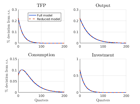
(optional) Step 7: Plot relevant values

Plot impulse response functions

plot_IRFs;

State Space Reduction with More Observables

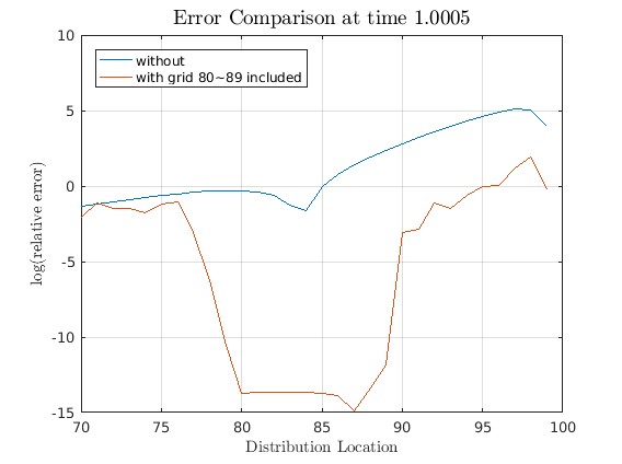
It is possible to include other variables into observables. In this part, different parts of the distribution will be included in the model reduction to show how the Krylov subspace based model reduction behaves. To that regard, the reduced model is solved while including different parts of distribution as part of the observable. In this case, a very strong requirement of knowing the probability density value at different grid points of the distribution g is taken. In the first case, 80th through 89th grid points were included in the parts that we consider to be observable. For the second example, 85th through 94th grid points were included in observable.

% rename derivative matrix to match notation in paper
g0 = mVarsDotDerivs;
g1 = -mVarsDerivs;
c = sparse(nVars,1);
psi = -mShocksDerivs;
pi = -mEErrorsDerivs;

% Solve full model
[~,inv_state_red,g0_full,g1_full,c_full,pi_full,psi_full] = clean_G0_sparse(g0,g1,c,pi,psi);
[G1,~,impact,eu] = schur_solver(g0_full,g1_full,c_full,psi_full,pi_full,1,1,1);
[simulated,vTime] = simulate(G1,impact,T,N,vAggregateShock,'implicit',inv_state_red);
simulated_full = simulated + varsSS;

% Solve reduced without extra observables
[state_red,inv_state_red,n_g_red] = krylov_reduction(g0,g1,n_v,n_g,20);
[g1_red,psi_red,pi_red,c_red,g0_red] = change_basis(state_red,inv_state_red,g1,psi,pi,c,g0);
[G1,~,impact,eu] = schur_solver(g0_red,g1_red,c_red,psi_red,pi_red,1,1,1);
[simulated,vTime] = simulate(G1,impact,T,N,vAggregateShock,'implicit',inv_state_red);
simulated_red = simulated + varsSS;

Solve reduced with extra observables for 80th through 89th grid point

[state_red,inv_state_red,n_g_red] = krylov_reduction(g0,g1,n_v,n_g,20,spdiags(ones(n_g,1),79,10,n_g));
[g1_80,psi_80,pi_80,c_80,g0_80] = change_basis(state_red,inv_state_red,g1,psi,pi,c,g0);
[G1,~,impact,eu] = schur_solver(g0_80,g1_80,c_80,psi_80,pi_80,1,1,1);
[simulated,vTime] = simulate(G1,impact,T,N,vAggregateShock,'implicit',inv_state_red);
simulated_obs = simulated + varsSS;
diff_red = (abs(simulated_red(n_v+1:end,:) - simulated_full(n_v+1:end,:)))./simulated_full(n_v+1:end,:);
diff_obs80 = (abs(simulated_obs(n_v+1:end,:) - simulated_full(n_v+1:end,:)))./simulated_full(n_v+1:end,:);

figure;
plot(70:99,log(diff_red(70:99,11)));
hold on;
plot(70:99,log(diff_obs80(70:99,11)));
grid on
legend('Location','northwest');
legend('without','with grid 80~89 included');
title(['Error Comparison at time ',num2str(vTime(11))],'interpreter','latex','fontsize',14)
ylabel('$\log$(relative error)','interpreter','latex')
xlabel('Distribution Location','interpreter','latex')

Solve reduced with extra observables for 85th through 94th grid point

[state_red,inv_state_red,n_g_red] = krylov_reduction(g0,g1,n_v,n_g,20,spdiags(ones(n_g,1),84,10,n_g));
[g1,psi,pi,c,g0] = change_basis(state_red,inv_state_red,g1,psi,pi,c,g0);
[G1,~,impact,eu] = schur_solver(g0,g1,c,psi,pi,1,1,1);
[simulated,vTime] = simulate(G1,impact,T,N,vAggregateShock,'implicit',inv_state_red);
simulated_obs = simulated + varsSS;
diff_obs = (abs(simulated_obs(n_v+1:end,:) - simulated_full(n_v+1:end,:)))./simulated_full(n_v+1:end,:);

figure;
plot(70:99,log(diff_red(70:99,11)));
hold on;
plot(70:99,log(diff_obs(70:99,11)));
grid on
legend('Location','northwest');
legend('without','with grid 85~94 included');
title(['Error Comparison at time ',num2str(vTime(11))],'interpreter','latex','fontsize',14)
ylabel('$\log$(relative error)','interpreter','latex')
xlabel('Distribution Location','interpreter','latex')

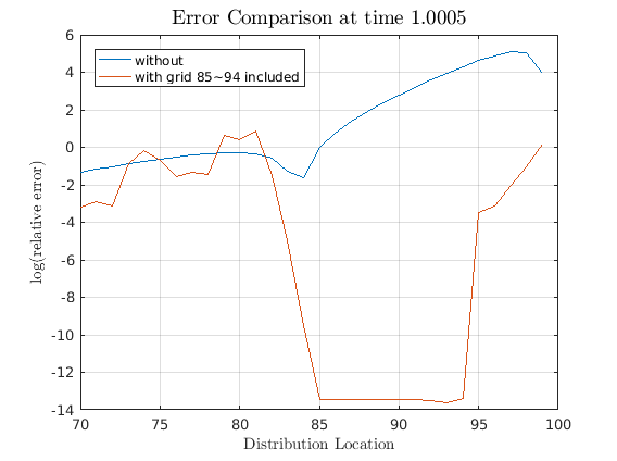
Note how the errors decreases only for the parts that we required to be observable while the irrelevant parts were reduced away. This is the magic of Krylov subspace based reduction in action. Though we could solve the full model for the simple Krusell-Smith case, this ability to reduce away irrelevant part will be essential for bigger problems.

Lastly, some of the functions have lengthy parameters, you can always type "help function_name;" to see documentation. All functions contain the function call syntax as the last line, and thoese can be copied and pasted into the program file. For example, to use the krylov_reduction function, you can call

help krylov_reduction;

  Reduce the dimensionality of state space using Krylov subspace method
 
  by SeHyoun Ahn, Sept 2016
 
  REFERENCE: Ahn, SeHyoun, Greg Kaplan, Benjamin Moll, Thomas Winberry, and
     Christian Wolf. "When Inequality Matters for Macro and Macro Matters
     for Inequality."
 
  PARAMETERS:
     g0 = LHS matrix, only used to check it satisfies require form
     g1 = Dynamics matrix
     n_v = number of jump variables
     n_g = number of state variables to be reduced
     n_Z = number of state variables not being reduced
     n_arnoldi = dimension of Krylov subspace
     varargin(1) = other observables
     varargin(2) = updating parameter for B_gv
     varargin(3) = number of variables to be NOT reduced; it is assumed
                   that the last varargin(3) variables are not being
                   reduced, so reorder as necessary
 
  OUTPUTS:
     state_red = tranformation to get from full grid to reduced states
     inv_state_red = inverse transform
     n_g_red = number of state variables after reduction
 
  SYNTAX:
  [state_red,inv_state_red,n_g_red] = krylov_reduction(g0,g1,n_v,n_g,n_arnoldi,varargin)

and just copy the lastline of the documentation string. Alternately, you can call "doc function_name" to read the doc string in the MATLAB help browser, and "edit function_name" to see the function codes.

Published with MATLAB® R2016b on 2017-04-05
    (and adjusted not to clash with Bootstrap)

SYSTEM INFORMATION FOR REPLICATION
Computer:
	Version: Lenovo IdeaPad Y400

CPU:
	Version: Intel(R) Core(TM) i7-3630QM CPU @ 2.40GHz

Memory:
	Number Of Devices: 2
Memory Device
	Size: 4096 MB
	Type: DDR3
	Speed: 1600 MHz
	Configured Clock Speed: 1600 MHz
Memory Device
	Size: 4096 MB
	Type: DDR3
	Speed: 1600 MHz
	Configured Clock Speed: 1600 MHz

MATLAB:
9.1.0.441655 (R2016b)