One-Asset HANK model

This program solves one-asset HANK model using the pertrubation method outlined in Ahn et al. (2017). The model setup is explained in more detail in the documentation file provided at </examples/one_asset_HANK/docs/one_asset_HANK.pdf> .

The solution will also follow the standard steps

Estimated Runtime: 1 ~ 2 seconds per solution This web run solves it 5 times run time depends heavily on internal consistency check that only needs to be run once afterward

REFERENCES:

REQUIRES:

Contents

Initialization

Setup the toolbox Need to include folders containing the files

addpath('/home/sehyoun/Dropbox/1Packages/PHACT');
addpath('/home/sehyoun/Dropbox/1Packages/AutoDiff');

% Turn off the warning message from auto diff
% You should read the warning once, but turn it off after reading it.
warning('off','AutoDiff:maxmin');

Set options for this example run

ReduceDistribution = 1;  % 1 for state space reduction 0 for not
reduceV = 1;             % 1 for value function reduction 0 for not
ReduceDist_hors = [25,30,35,40];     % Dimensionality of the Krylov subspace
DisplayLev = 1;          % Determines verbosity of steady state calculation
check_consistency = 1;   % Runs Step 6: Internal consistency check

Step 0: Set parameters

Run script to setup parameters Economic parameters, approximation parameters, and grid parameters are defined in the script.

set_parameters;

n_v = I*J + 1;          % number of choice/jump variables (value function + inflation)
n_g = I*J;              % number of state variables (distribution + monetary policy)
n_p = 5;                % number of static relations (includes observables)
n_shocks = 1;           % only monetary policy shock is considered
nEErrors = n_v;
nVars = n_v + n_g + n_p;

Step 1: Solve for the Steady State

Any methods can be used to solved for the steady state. In particular, example codes can be found at <http://www.princeton.edu/~moll/HACTproject.html>.

fprintf('Computing steady state...\n');
t0 = tic;
compute_steady_state;
fprintf('Time to compute steady state: %2.4f seconds\n\n\n',toc(t0));

Computing steady state...
Discount rate: 0.02, Excess Demand: -5.7787
Discount rate: 0.0125, Excess Demand: -5.4142
Discount rate: 0.00875, Excess Demand: -4.8266
Discount rate: 0.006875, Excess Demand: -4.0908
Discount rate: 0.0059375, Excess Demand: -3.1858
Discount rate: 0.0054687, Excess Demand: -2.0309
Discount rate: 0.0052344, Excess Demand: -0.57438
Discount rate: 0.0051172, Excess Supply: 1.3215
Discount rate: 0.0051758, Excess Supply: 0.14704
Discount rate: 0.0052051, Excess Demand: -0.24977
Discount rate: 0.0051904, Excess Demand: -0.061274
Discount rate: 0.0051831, Excess Supply: 0.040435
Discount rate: 0.0051868, Excess Demand: -0.011263
Discount rate: 0.0051849, Excess Supply: 0.014417
Discount rate: 0.0051859, Excess Supply: 0.0015324
Discount rate: 0.0051863, Excess Demand: -0.0048544
Discount rate: 0.0051861, Excess Demand: -0.0016539
Discount rate: 0.005186, Excess Demand: -5.6366e-05
Discount rate: 0.0051859, Excess Supply: 0.0007432
Discount rate: 0.0051859, Excess Supply: 0.0003423
Discount rate: 0.005186, Excess Supply: 0.00014249
Discount rate: 0.005186, Excess Supply: 4.2562e-05
Steady State Found, Interest rate = 0.005, Discount rate = 0.005186
Time to compute steady state: 0.4049 seconds

Step 2: Linearize Model Equations

For computing derivatives, the codes written for solving for the steady-state can be used almost verbatim using automatic differentiation toolbox as long as only the functions supported by automatic differentation are used. For list of supported functions and documentation of relevant syntax check <https://github.com/sehyoun/MATLABAutoDiff>. Example usage/syntax of automatic differentiation can be found at <https://sehyoun.com/EXAMPLE_AutoDiff_Syntax.html>.

fprintf('Taking derivatives of equilibrium conditions...\n');
t0 = tic;

% Prepare automatic differentiation
vars = zeros(nVars + nVars + nEErrors + n_shocks,1);
vars = myAD(vars);

% Evaluate derivatives
equilibrium_conditions;

% Extract derivative values
derivs = getderivs(v_residual);

t_derivs = toc(t0);
fprintf('Time to compute derivatives: %2.4f seconds\n\n\n',t_derivs);
if t_derivs> 1
    warning('If you do not compile mex/C files for the automatic differentiation, matrix vector multiplication will be slow');
    disp('Press any key to continue...');
    pause();
end

Taking derivatives of equilibrium conditions...
Time to compute derivatives: 0.1139 seconds

Step 3: Solve out Static Constraints or Reduce the Model

Extract derivatives

g1 = -derivs(:,1:nVars);
g0 = derivs(:,nVars+1:2*nVars);
pi = -derivs(:,2*nVars+1:2*nVars+nEErrors);
psi = -derivs(:,2*nVars+nEErrors+1:2*nVars+nEErrors+n_shocks);
constant = sparse(nVars,1);

% Solve out static constraints
fprintf('Solving Out Static Constraints ...\n');
[state_red,inv_state_red,g0,g1,constant,pi,psi] = clean_G0_sparse(g0,g1,constant,pi,psi);
n_g_red = n_g;

% Create identity matrix for code reuse below
from_spline = speye(n_g_red + n_v);
to_spline = speye(n_g_red + n_v);
n_splined = n_v;

Solving Out Static Constraints ...

Step 4: Solve Linear Systems

t0 = tic;
fprintf('Solving linear system...\n');

% Note parts of schur_solver will be swapped out in the
%    near future, so it might have a different interface. Since the codebase is
%    new, there will be interative updates to simplify interface and syntax.
%    Underlying math will stay the same, but interfact may change with updates,
%    so one should note the release number of the codebase one is using.
[G1, ~, impact, eu, F] = schur_solver(g0,g1,c,psi,pi,1,1,1,n_splined);
fprintf('...Done!\n')
fprintf('Existence and uniqueness? %2.0f and %2.0f\n',eu);
fprintf('Time to solve linear system: %2.4f seconds\n\n\n',toc(t0));

Solving linear system...
...Done!
Existence and uniqueness?  1 and  1
Time to solve linear system: 0.0390 seconds

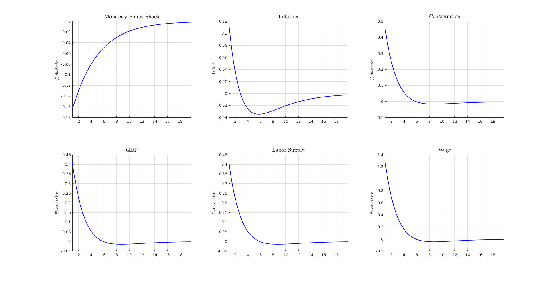
Step 5: Simulate Impulse Response Functions

fprintf('Simulating Model...\n');
t0 = tic;

T = 100;
N = 400;
dt = T/N;
vAggregateShock	= zeros(1,N);
vAggregateShock(1) = -1/sqrt(dt);
trans_mat = inv_state_red*from_spline;
[simulated,vTime] = simulate(G1,impact,T,N,vAggregateShock,'implicit',trans_mat,[n_v,n_v+n_g:n_v+n_g+5]);

fprintf('...Done!\n');
fprintf('Time to simulate model: %2.4f seconds\n\n\n',toc(t0));

% Define variables to be plotted below
inflation = simulated(1,:)';
monetary_shock = simulated(2,:)';
consumption = (simulated(4,:)')/vars_SS(n_v+n_g+3);
Y = (simulated(6,:)')/vars_SS(n_v+n_g+4);
lab_sup = (simulated(4,:)')/vars_SS(n_v+n_g+2);
wage = simulated(3,:)'/vars_SS(n_v+n_g+1);

Simulating Model...
...Done!
Time to simulate model: 0.0121 seconds

(optional) Step 7: Plot relevant IRFs

fig = figure('units','normalized','outerposition',[0 0 1 1]);
line_style = '-';
color = 'blue';
plot_IRFs;

Step 3: Reduce the Model

Now, the model will be solved again using model reduction (4 times) However, the code steps through similar steps as above except with reduction.

ReduceDist_hor = ReduceDist_hors(1);
fprintf('\n\nReduction horizon %d\n',ReduceDist_hor);
g1 = -derivs(:,1:nVars);
g0 = derivs(:,nVars+1:2*nVars);
pi = -derivs(:,2*nVars+1:2*nVars+nEErrors);
psi = -derivs(:,2*nVars+nEErrors+1:2*nVars+nEErrors+n_shocks);
constant = sparse(nVars,1);

% State Variables
% Reduce model
fprintf('Reducing distribution ...\n');
[state_red,inv_state_red,n_g_red] = krylov_reduction(g0,g1,n_v,n_g,ReduceDist_hor);
[g1,psi,pi,constant,g0] = change_basis(state_red,inv_state_red,g1,psi,pi,constant,g0);
fprintf('Reduced to %d from %d.\n',n_g_red,n_g);

% Jump Variables
% Reduce dimensionality of value function using splines
n_knots = 15;
c_power = 1;
x = a';
n_post = size(z,2);
n_prior = 1;

% Create knot points for spline (the knot points are not uniformly spaced)
knots = linspace(amin,amax,n_knots-1)';
knots = (amax-amin)/(2^c_power-1)*((knots-amin)/(amax-amin)+1).^c_power+ amin-(amax-amin)/(2^c_power-1);

% Function calls to create basis reduction
[from_spline, to_spline] = oneDquad_spline(x,knots);
[from_spline, to_spline] = extend_to_nd(from_spline,to_spline,n_prior,n_post);
from_spline(end+1,end+1) = 1;
to_spline(end+1,end+1) = 1;
n_splined = size(from_spline,2);
[from_spline, to_spline] = projection_for_subset(from_spline,to_spline,0,n_g_red);

% Reduce the decision vector
[g1,psi,~,constant,g0] = change_basis(to_spline,from_spline,g1,psi,pi,constant,g0);
pi = to_spline * pi * from_spline(1:n_v,1:n_splined);

Reduction horizon 25
Reducing distribution ...
Reduced to 50 from 100.

Step 4: Solve Linear Systems

t0 = tic;
fprintf('Solving linear system...\n');

% Note parts of schur_solver will be swapped out in the
%    near future, so it might have a different interface. Since the codebase is
%    new, there will be interative updates to simplify interface and syntax.
%    Underlying math will stay the same, but interfact may change with updates,
%    so one should note the release number of the codebase one is using.
[G1, ~, impact, eu, F] = schur_solver(g0,g1,c,psi,pi,1,1,1,n_splined);
fprintf('...Done!\n')
fprintf('Existence and uniqueness? %2.0f and %2.0f\n',eu);
fprintf('Time to solve linear system: %2.4f seconds\n\n\n',toc(t0));

Solving linear system...
Warning: <schur_solver>: There are less than n_v number of positive eigenvalues: 
   -0.0012

...Done!
Existence and uniqueness?  1 and  1
Time to solve linear system: 0.0050 seconds

Step 5: Simulate Impulse Response Functions

fprintf('Simulating Model...\n');
t0 = tic;

T = 100;
N = 400;
dt = T/N;
vAggregateShock	= zeros(1,N);
vAggregateShock(1) = -1/sqrt(dt);
trans_mat = inv_state_red*from_spline;
[simulated,vTime] = simulate(G1,impact,T,N,vAggregateShock,'implicit',trans_mat,[n_v,n_v+n_g:n_v+n_g+5]);

fprintf('...Done!\n');
fprintf('Time to simulate model: %2.4f seconds\n\n\n',toc(t0));

% Define variables to be plotted below
inflation = simulated(1,:)';
monetary_shock = simulated(2,:)';
consumption = (simulated(4,:)')/vars_SS(n_v+n_g+3);
Y = (simulated(6,:)')/vars_SS(n_v+n_g+4);
lab_sup = (simulated(4,:)')/vars_SS(n_v+n_g+2);
wage = simulated(3,:)'/vars_SS(n_v+n_g+1);

Simulating Model...
...Done!
Time to simulate model: 0.0062 seconds

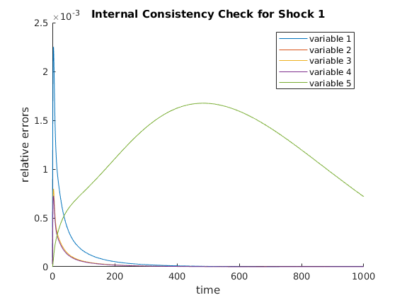
Step 6: Internal Consistency Check

A different internal consistency check will be implemented and updated in the future. This function should only be taken as a sanity check.

g1 = -derivs(:,1:nVars);
psi = -derivs(:,2*nVars+nEErrors+1:2*nVars+nEErrors+n_shocks);
from_red = inv_state_red * from_spline;
to_red = to_spline * state_red;
[epsilon] = internal_consistency_check(G1,impact,n_g_red,from_red,to_red,g1,psi,F,n_v,n_g,1000,vars_SS,1,0.07);

<check_internal>: Estimated simulation time is 0.402892 minutes
<internal_consistency_check>: The maximum relative error is 2.251858e-03

(optional) Step 7: Plot relevant IRFs

figure(fig);
line_style = '--';
color = 'red';
plot_IRFs;

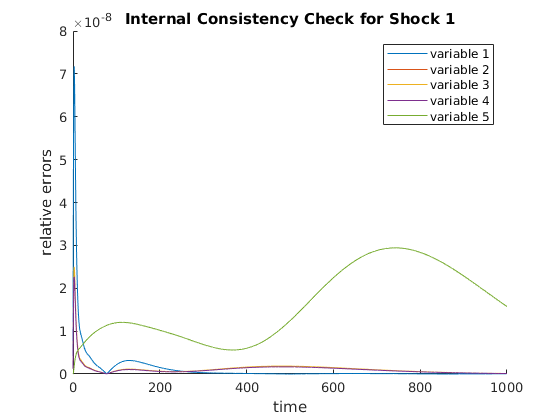
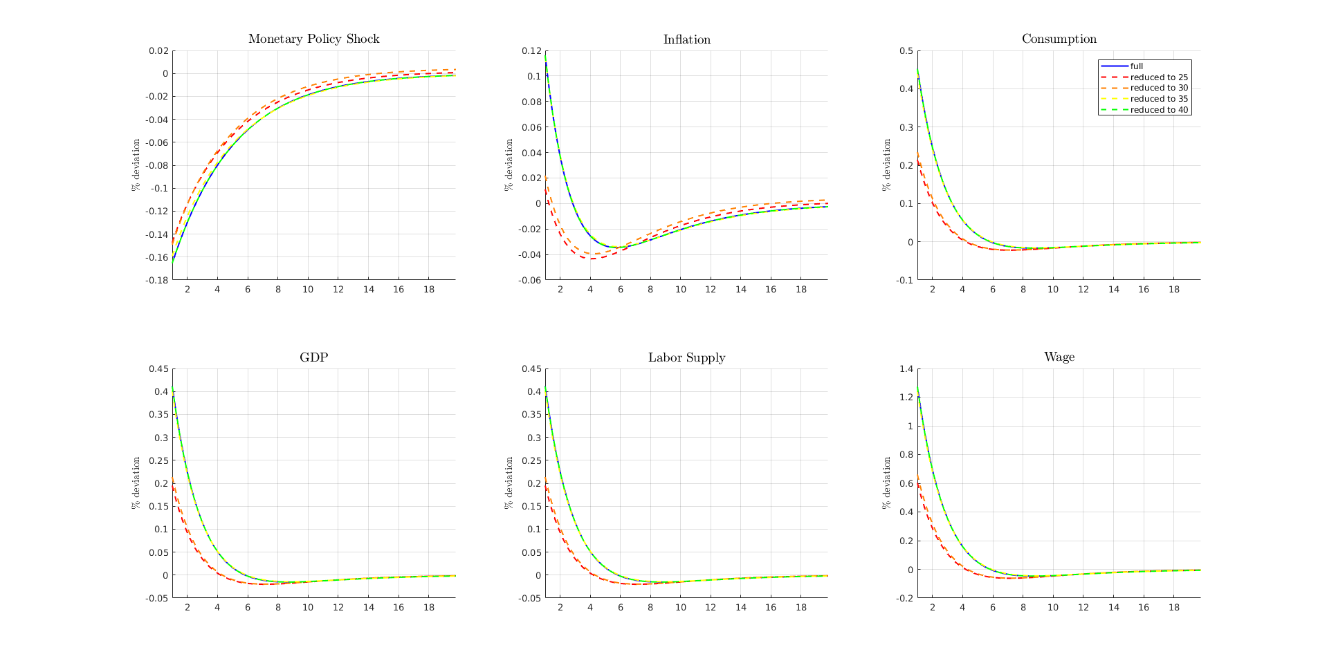
Repeatly Solve the Reduced Model 3 more times with different Krylov order

Above codes are delegated to <solve_reduced_model> script for cleanliness.

ReduceDist_hor = ReduceDist_hors(2);
fprintf('\n\nReduction horizon %d\n',ReduceDist_hor);
color = [1,0.5,0];
solve_reduced_model;

ReduceDist_hor = ReduceDist_hors(3);
fprintf('\n\nReduction horizon %d\n',ReduceDist_hor);
color = 'yellow';
solve_reduced_model;

ReduceDist_hor = ReduceDist_hors(4);
fprintf('\n\nReduction horizon %d\n',ReduceDist_hor);
color = 'green';
solve_reduced_model;

legends = cell(5,1);
legends{1} = 'full';
legends{2} = ['reduced to ',num2str(ReduceDist_hors(1))];
legends{3} = ['reduced to ',num2str(ReduceDist_hors(2))];
legends{4} = ['reduced to ',num2str(ReduceDist_hors(3))];
legends{5} = ['reduced to ',num2str(ReduceDist_hors(4))];

figure(fig);
subplot(2,3,3);
legend(legends{:});

Reduction horizon 30
Reducing distribution ...
Reduced to 60 from 100.
Solving linear system...
Warning: <schur_solver>: There are less than n_v number of positive eigenvalues: 
  -4.4176e-04

...Done!
Existence and uniqueness?  1 and  1
Time to solve linear system: 0.0064 seconds


Simulating Model...
...Done!
Time to simulate model: 0.0069 seconds


<check_internal>: Estimated simulation time is 0.398945 minutes
<internal_consistency_check>: The maximum relative error is 2.667717e-03


Reduction horizon 35
Reducing distribution ...
Reduced to 70 from 100.
Solving linear system...
...Done!
Existence and uniqueness?  1 and  1
Time to solve linear system: 0.0091 seconds


Simulating Model...
...Done!
Time to simulate model: 0.0076 seconds


<check_internal>: Estimated simulation time is 0.506851 minutes
<internal_consistency_check>: The maximum relative error is 1.528743e-03


Reduction horizon 40
Reducing distribution ...
Reduced to 80 from 100.
Solving linear system...
...Done!
Existence and uniqueness?  1 and  1
Time to solve linear system: 0.0076 seconds


Simulating Model...
...Done!
Time to simulate model: 0.0068 seconds


<check_internal>: Estimated simulation time is 0.400918 minutes
<internal_consistency_check>: The maximum relative error is 7.174923e-08

Published with MATLAB® R2017a on 2017-10-17
    (and adjusted not to clash with Bootstrap)

SYSTEM INFORMATION FOR REPLICATION
Computer:
	Version: ThinkPad P50

CPU:
	Version: Intel(R) Xeon(R) CPU E3-1505M v5 @ 2.80GHz

Memory:
	Number Of Devices: 4
Memory Device
	Size: 16384 MB
	Type: DDR4
	Speed: 2133 MHz
	Configured Clock Speed: 2133 MHz
Memory Device
	Size: 16384 MB
	Type: DDR4
	Speed: 2133 MHz
	Configured Clock Speed: 2133 MHz
Memory Device
	Size: 16384 MB
	Type: DDR4
	Speed: 2133 MHz
	Configured Clock Speed: 2133 MHz
Memory Device
	Size: 16384 MB
	Type: DDR4
	Speed: 2133 MHz
	Configured Clock Speed: 2133 MHz

OS:
Description:	Linux Mint 18.1 Serena

MATLAB:
9.2.0.556344 (R2017a)

REFERENCES:

- Ahn, SeHyoun, et al. "When Inequality Matters for Macro and Macro Matters for Inequality." NBER Macroeconomics Annual 2017, volume 32. University of Chicago Press, 2017.
- Kaplan, Greg, Benjamin Moll, and Giovanni L. Violante. Monetary policy according to HANK. No. w21897. National Bureau of Economic Research, 2016.
REQUIRES:
- auto diff toolbox: <https://github.com/sehyoun/MATLABAutoDiff>
- phact toolbox: <https://github.com/gregkaplan/phact>
- <compute_steady_state.m>
- <equilibrium_conditions.m>
- <set_parameters.m>