Steady-State Distribution of Ornstein-Uhlenbeck Process
Expected Read Time: 4~7 minutes
In this tutorial, we will solve for the distribution of resulting from the Ornstein-Uhlenbeck Process
in 2-dimension. From an explicit calculation, one can get that the steady-state is given by
Since the actual program itself is not long, we will carry everything. First, we define the parameters of the Ornstein-Uhlenbeck process
>> n_dim = 2;
>> n_points = 20;
>> int_sig = 0.1;
>> make_plots = true;

>> mu = 0.495.*ones(1, n_dim);
>> theta = 1.*ones(n_dim,1);
>> sigma = int_sig.^2.*ones(n_dim, 1);
Hence, we have
To implement this example, we initialize the afv_grid object.
>> grid = afv_grid(2);
First, we will split the grid uniformly into 20 grid points using split_init. This function only allows tensor structure division of the grid (regular grid), and the splitting cut points are given as cells of vectors of dimension.
>> cut_points = cell(n_dim, 1);
>> cut_points_1d = linspace(0, 1, n_points+1);
>> cut_points_1d = cut_points_1d(2:end-1)';
>> for iter_dim = 1:n_dim
>>     cut_points{iter_dim} = cut_points_1d;
>> end
>> grid.split_init(1, cut_points);
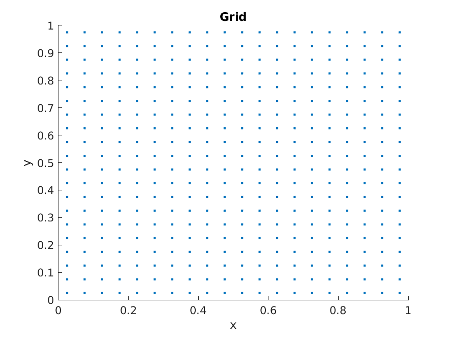
At this points, [0,1]x[0,1] has been split into 400 grid points (20 per dimension). We can visualize this by making a scatter plot of center of the cells. One can compute the center of the cells via node_midpoints.
>> x_i = grid.node_midpoints();
>> scatter(x_i(:,1), x_i(:,2));
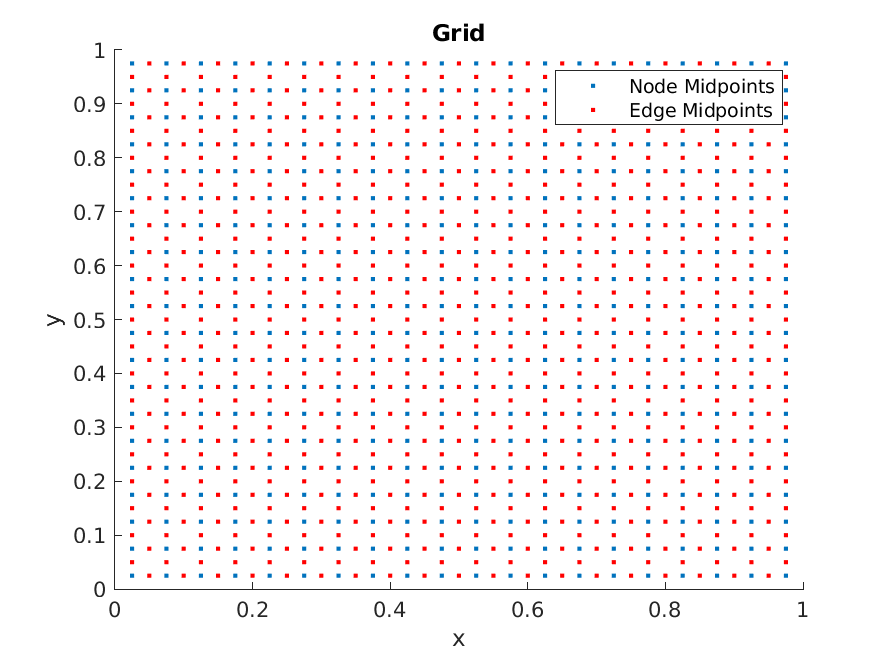
At this point, the grid only has the information on the cells. It keeps the neighbor structure of the cells updated, but not the edges. The edge information can be updated via extract_edges. Whenever the grid structure changes, extract_edges needs to be called to make sure that the edge structure is consistent with the updated grid.
>> grid.extract_edges();
We can visualize edges by making a scatter plot of their midpoints (using edge_midpoints) as well
>> hold on;
>> x_i = grid.edge_midpoints();
>> scatter(x_i(:,1), x_i(:,2), 'r.');
Now, we are ready to implement the Ornstein-Uhlenbeck process. The equation is completely defined with drifts and diffusion terms corresponding to the edges. The data for edges are stored as a vector. However, the drift values needs to be different depending on which direction the edge faces. The normal direction of the edge are stored as e2dir. Hence, the drift terms can be implemented with
>> x_i = grid.edge_midpoints();
>> for iter_dim = 1:n_dim
>>     cur_ind = find(grid.e2dir(1:grid.num_e) == iter_dim);
>>     grid.drift(cur_ind) = -theta(iter_dim).*(x_i(cur_ind, iter_dim) - mu(iter_dim));
>> end
For example, with iter_dim = 1, the drift value of the edges facing the first coordinate directions are updated. This is why \(x_1\) ( = x_i(cur_ind, iter_dim) ) is used to compute the drift.
Diffusions can be implemented in a similar manner:
>> for iter_dim = 1:n_dim
>>     cur_ind = find(grid.e2dir(1:grid.num_e) == iter_dim);
>>     grid.diffusion(cur_ind) = sigma(iter_dim);
>> end
Note that the value that’s defined for diffusion is \(\sigma^2_i\), without the factor \(\frac{1}{2}\). As the fraction \(\frac{1}{2}\) shows up in all equations, it is taken as implicit when the transition matrix is built.
Now, once we have set the drift and diffusion terms to the edges, we can build the transition matrix using compute_transition_matrix_modified.
>> A = grid.compute_transition_matrix_modified();
For the steady-state, we find a solution to \(Ag = 0\). Hence, we can use any eigenvalue solver to do so.
>> [g, ~] = eigs(A_FP, 1, 'sm');
>> g = g./sum(g);
Finally, we can make a plot to see the accuracy of the scheme
>> x_i = grid.node_midpoints();
>> scatter3(x_i(:,1),x_i(:,2),g./grid.node_weights);
>> hold on;
>> scatter3(x_i(:,1),x_i(:,2),g_true(x_i),'.');
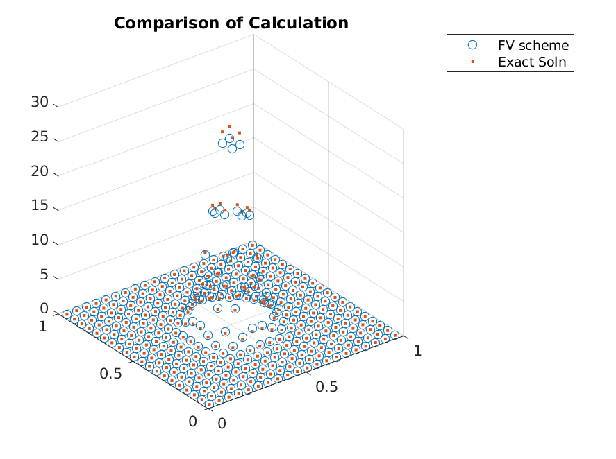
For this particular set of parameters, the grid is not good enough to approximate with high accuracy. One can see that this is largely due to picking wrong domain for the parameter values. This will be fixed by adjusting domain or using adaptive refinements. The adaptive refinements will be shown in the next tutorial, but in the mean time, let’s solve a problem with nicer parameters.
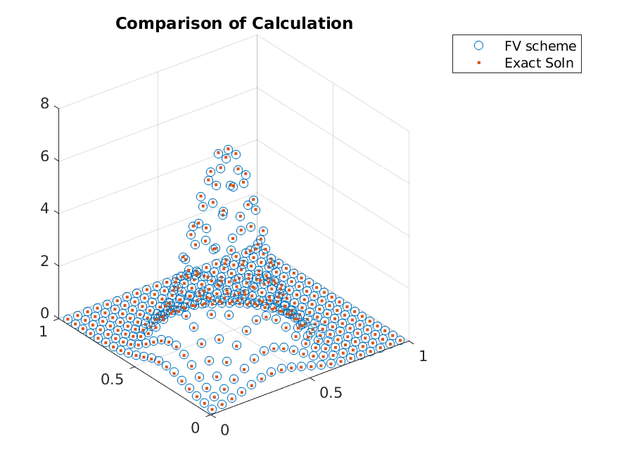
Updating to a new parameters highlights one nice feature of the finite volume discretization. With the finite volume method, the structure of the transition matrix is independent of the parameter values, so only the drift and diffusion have to be updated to reflect the new parameters.
To implement these parameters, we can just update the drifts and diffusion
>> int_sig = 0.2;
>> make_plots = true;

>> mu = 0.35.*ones(1, n_dim);
>> theta = 1.*ones(n_dim,1);
>> sigma = int_sig.^2.*ones(n_dim, 1);

>> x_i = grid.edge_midpoints();
>> for iter_dim = 1:n_dim
>>     cur_ind = find(grid.e2dir(1:grid.num_e) == iter_dim);
>>     grid.drift(cur_ind) = -theta(iter_dim).*(x_i(cur_ind, iter_dim) - mu(iter_dim));
>>     grid.diffusion(cur_ind) = sigma(iter_dim);
>> end
and compute the transition matrix and the steady-state distribution
>> A = grid.compute_transition_matrix_modified();
>> [g, ~] = eigs(A_FP, 1, 'sm');
>> g = g./sum(g);
To conclude, one can implement the finite volume method follow a simple recipe. One just needs to call
- Initialize grid
afv_grid- Split the grid
split_init- Extract Edges
extract_edges- Define drifts and diffusion
- Build transition matrix
compute_transition_matrix_modified
Technical Disclaimer: In the tutorial there was no mention of the boundary conditions. Implicitly it is being assumed that the boundary is a reflecting boundary. Hence, if \(\sigma_i\)‘s are too large, the exact solution is not the exact solution to the PDE being solved by the finite-volume method. Allowing “flows” at the boundaries will be considered later (compute_transition_matrix_boundary.)